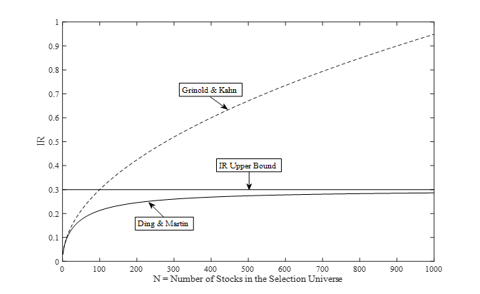
The generalized fundamental law of active management
The generalized fundamental law of active management establishes the underlying relationship between expected portfolio performance (IR) and the portfolio characteristics based on bets on quantitative factors such as momentum, value, etc. It extends the work by Grinold and Kahn to the more interesting case where factor information coefficients (ICs) are time-varying.
Let’s say an investor wants to build a long-short dollar neutral portfolio by betting on stocks with high momentum, and shorting stocks with low momentum from a selection universe with N stocks, what will be her/his expected portfolio information ratio (IR)? The answer is the generalized fundamental law of active management:
![\[ \text{IR} = \frac{{\mu}_{\text{IC}}}{\sqrt{(1-{\mu}_{\text{IC}}^2-{\sigma}_{\text{IC}}^2)/N+{\sigma}_{\text{IC}}^2}} \approx \frac{{\mu}_{\text{IC}}}{{\sigma}_{\text{IC}}} \]](https://alphafocusir.com/wp-content/ql-cache/quicklatex.com-eb47e1ccd14ac909d2cc9e2c33fd3f4d_l3.png "Rendered by QuickLaTeX.com")
where  is the mean IC (Information Coefficient, correlation) between risk adjusted stock excess returns and risk adjusted factor exposures,
  is the IC standard deviation.
Figure 1. The fundamental law of active management
 and
and  .
.![\[ \text{IR} = {\sqrt{{\boldsymbol{\mu}_{\text{IC}}^'} ({\sigma}_{\epsilon}^2/N {\mathbf{I}}+{\boldsymbol{\Sigma}}_{\text{IC}})^{-1}{\boldsymbol{\mu}}_{\text{IC}}}} \approx \sqrt{{{\boldsymbol {\mu}}_{\text{IC}}^'}{\boldsymbol{\Sigma}}_{\text{IC}}^{-1}{\boldsymbol{\mu}}_{\text{IC}}}} \]](https://alphafocusir.com/wp-content/ql-cache/quicklatex.com-f6ed0d5643ec2c0ad21273114ec0c0c5_l3.png "Rendered by QuickLaTeX.com")
 is the mean Information Coefficient vector (correlation) between risk adjusted stock excess returns and risk-adjusted factor exposures,
  is the factor IC covariance matrix.
![\[ {\mathbf{w}_{A,t}} = {\frac{1}{N}} {\boldsymbol{\Lambda}}_t^{-1/2} {\mathbf{Z}}_{t-1}{\frac{{{\sigma}_A}{\boldsymbol{\Sigma}}_{\text{IC}}^{-1}{\boldsymbol{\mu}}_{\text{IC}}}{\sqrt{{{\boldsymbol {\mu}}_{\text{IC}}^'}{\boldsymbol{\Sigma}}_{\text{IC}}^{-1}{\boldsymbol{\mu}}_{\text{IC}}}}}} ={\frac{1}{N}} {\boldsymbol{\Lambda}}_t^{-1/2} {\mathbf{Z}}_{t-1}{\mathbf{w}_f}={\left({\frac{1}{N{\sigma}_{r_{it}}}}\sum_{k=1}^{K}{{w_{f,k}}{z_{ik,t-1}}}\right)}_{i=1,\ldots,N} \]](https://alphafocusir.com/wp-content/ql-cache/quicklatex.com-ac1cc58dd53c7c6a5b60531b727573a3_l3.png "Rendered by QuickLaTeX.com")
![\[ {\mathbf{w}_f} = {\frac{{{\sigma}_A}{\boldsymbol{\Sigma}}_{\text{IC}}^{-1}{\boldsymbol{\mu}}_{\text{IC}}}{\sqrt{{{\boldsymbol {\mu}}_{\text{IC}}^'}{\boldsymbol{\Sigma}}_{\text{IC}}^{-1}{\boldsymbol{\mu}}_{\text{IC}}}}}} \]](https://alphafocusir.com/wp-content/ql-cache/quicklatex.com-a6b90cda11dc174d490486e8aae7db55_l3.png "Rendered by QuickLaTeX.com")
 . The factor weight times each stock’s corresponding factor exposure, divided by each stock’s volatility, gives the optimal portfolio’s stock weight.
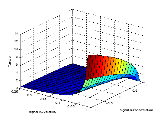
![\[ \text{TO} = \frac{{\sigma}_A \sqrt{1-{\rho}_z}}{\sqrt{\pi} \sqrt{(1-{\mu}_{\text{IC}}^2-{\sigma}_{\text{IC}}^2)/N+{\sigma}_{\text{IC}}^2}} E_{cs}{\left(\frac{1}{{\sigma}_{r_i}}\right)} \]](https://alphafocusir.com/wp-content/ql-cache/quicklatex.com-4540ccfe7443ee802fbe4795404951c7_l3.png "Rendered by QuickLaTeX.com")
 , inversely correlated with factor IC standard deviation and average individual security volatility, and positively related to portfolio tracking error